How do I get the ruler back in Word 2007?

Wondering what happened to the ruler accross the top of your page in Word 2007? In order to show/hide the horizontal ruler, you need to click on the tiny little "view ruler" icon on the right of your document (I've highlight it above).

The vertical rulers should also come on by default, but if not this must be changed through Word Options. To access this select the main Office button>Word Options.

Select Advanced and then scroll down to Display. Here you will notice an option to turn vertical ruler on when in print layout view. Make sure there is a tick next to this.

Now you can turn all your rulers on and off as needed when in print layout simply by clicking the little ruler icon at the top of your right scroll bar.

How do I quickly see which cells I have used in a formula?

Excel 2007 has a few handy functions to find what cell's you have used in a formula. The quickest and simplest method is through the ribbon. On the formulas tab, above the heading Formula Auditing, you'll find Trace Precedents and Trace Dependents.





Precedents affect the value of the currently selected cell.
Dependents are those cells affected by the currently selected cell.

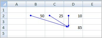
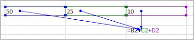
In the example below I have summed the values B2:D2 in cell D4. If I select D4 and click Trace Precedents, Excel will display blue arrows from the cells that affect the formula in this one. This can be a great help when you are dealing with a lot of data on the sheet.

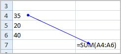
Determining dependents is just as simple. Below, I have select cell A4 and clicked Trace Dependents. A blue arrow appears from A4 to let me know that the formula in B7 is dependent upon this cell.


Tracing cell precedents and dependents can be a great way to view the relationships between values and quickly identify any origiins of errors.

How do I use Excel's IF function for simple look-ups?

The IF function is a versatile tool in Excel. You can use the IF function for simple lookups, such as returning certain numbers with specified text. Watch the demonstration below to see just how simple it is or scroll down for an overview. Example from John Walkenbach's Excel 2007 Bible.

In the Excel sheet below I have 10 student names in column A and their final marks in column B. To determine the grades in column C, I would type the following into cell C2:


=IF(B2>=50, "PASS", FAIL")

This tells Excel to return the text 'pass' if a student's mark is greater than or equal to 50, otherwise return a 'fail.' Once you have filled in the first cell with your formula, simply fill down the rest of the column.

Excel also allows you to nest IF functions to provide even more choices. In the table above, I have typed into cell c2:


=IF(B2<=49, "FAIL", IF(B2<=74, "GOOD", IF(B2<=84, "GREAT", IF(B2>84, "OUTSTANDING"))))

How do I get a large letter at the start of a paragraph in Word?

This is known as a drop cap. You have probably seen drop caps in books and magazines before. Drop caps can be an attractive decorative addition to your page and help to break up the text.

To use drop cap in Word 2007, select the Insert tab on the Word ribbon. Glance across the ribbon until you come to the Text menu options and locate Drop Cap (see image below).


Click the little down arrow in order to bring up the Drop Cap options. You can insert your drop cap dropped into your text (as seen at the top of this post) or place it into the margin area.

You will also notice that you can select Drop Cap Options. This allows you to select the font of your letter, choose how many lines to drop it and how far spaced from the other text you want your drop cap to be.

Have fun playing with the different fonts styles to create very different looks and feels to your documents.

How do I enable check boxes to select files in Vista?

One of my favourite Vista options is the ability to enable checkboxes in order to select files and folders in Explorer. Here's how you do it:

1. Click the Organize button at the top left of your explorer screen and scroll down to select Folder and Search Options (see image below).

2. Click on the View tab and scroll down until you come to the option Use Check Boxes to Select Items. Place a tick next to the option and Apply>Ok.

That's all there is to it! If you would like to see a visual demonstration of this process and the end result, have a look at the video below (my apologies as the audio quality is not as great I would have liked it).

How do I ensure Word updates linked data before printing?

I can't tell you how many times I have been typing up a project in Word that has newly changed linked Excel data and I have hit the print button before I update the information in my Word document. It's frustrating to say the least!

To prevent this hapenning, Word 2007 has a great setting you can use to ensure your linked data is updated before printing. If only I had found it sooner.

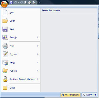
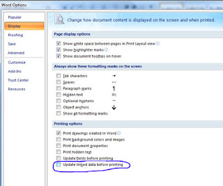
In Word 2007, click the Office button (that's the big multi-coloured one). At the bottom of the main menu you will notice a button called Word Options (see image below). Click this to bring up your settings.

With Word options now open, look down the left-hand side to select Display. Display options allow you to control how Word presents your document on screen and in print.

Under printing options, place a check in the final option box which says 'Update Linked Data Before Printing.' Select OK.

If you link data into your Word documents, this can be a great option to prevent accidental printing before updates.

How do I copy column widths in Excel?

One of the annoying and time-consuming things about Excel in the past has been the need to set up column widths on each sheet of a workbook. When you copied information accross, the columns widths didn't replicate themselves and you had to format them all over again.

The good news is that those days are over. Excel does allow you to copy and paste your column widths, saving time and keeping everything uniform.

Once you have the columns set up on a sheet you want to have the same widths in other sheets, simply select the columns and copy. Head to the sheet you want to paste those widths into. Instead of the paste command use Paste Special. The Paste Special dialogue box will appear as shown below.

You will notice that there is an option to paste Column Widths. Select this and click OK. Now you can quickly pre-format all the column widths in your worksheet!

How do I revert back to the old pivot table layout?

If you open your Excel 2007 in order to create a Pivot Table, you will no doubt be faced with the new layout (pictured above).

If you feel more comfortable using Excel's familiar pivot table layout, you can alter your settings to show the older style pivot table drag and drop box (pictured below).

To enable the previous version's look, select Pivot Table Tools> Pivot Table Options > Options. When the options box opens, click on the Display tab. Place a check into the box next to Classic Pivot Table Layout.

Now you have all the new functionality with an old faithful look and feel.

How do I create pivot tables in Excel 2007?

Pivot tables are an excellent way of organising large amounts of data, customised to suit your present needs. The pivot table layout is a little different in Excel 2007, but you'll soon find it has really improved and pivot tables are easier to use than ever before. Example from John Walkenbach's Excel 2007 Bible.

I'll include specific written instructions at a later time. For now, the best way to show you just how pivot tables are created is via the above video demonstration.

How do I make a thermometer chart in Excel?

A thermometer chart is a great way of visually showing the percentage of task that is completed or progress towards a specific goal. View the video demonstration below to learn how to create your own thermometer chart in Excel 2007.

What you will need to do is create a chart that uses a single cell reference as a data series (this will be your percentage).

You will then do a little formatting and tweaking of the Data Series (gap width to zero) and Axis options (minimum zero and maximum 1). Insert a textbox and link it to your percentage value (insert > textbox> (draw box where you want it) > F2 > =(select % value cell).

The rest is just cosmetic and you can play around with Excel's formatting options to suit yourself.

How do I add pictures to my chart in Excel?

Customising your excel charts with pictures is a fun and simple process. You can chose to have a picture background, picture plot area or even picture columns. See the video demonstration eblow or scroll down for a few basic instructions. Example from John Walkenbach's Excel 2007 Bible.

Background or plot area picture: Left click into the chart (or plot area only) to select it and then right click to bring up the menu. Choose Format Chart Area (or Format Plot Area if you are only adding the picture behind the series). Under fill options, select Picture or Texture Fill.

Insert from file to browse for the location of the picture on your computer and select the image you require. You can now make any stretch or transparency adjustments as you see fit. Close. There you have a picture background!

Columns as picture: Left click onto the columns in order to select them and right click to bring up the menu. Choose Format Data Series > Fill > Picture or Texture Fill > Insert From File. Locate the image on your computer and select it.

Several options are available to stretch the image, stack the image or scale it. Adjust these as suits your needs. Close. Now you have picture columns!

How do I open a group of favourite sites together?

Adding tab groups to your favourites is a great way to quickly access what you need. Once you have set up your tab group favourites, all pages in a group will open simultanously.

I like tab group favourites for projects that require me to frequent the same few sites. If you shop online, you can add your favourite stores into a tabbed group to open together when you're ready to browse.

From the menu choose Favourites > Add Tab Group to Favourites. Type in a folder name for the group (Fave Stores, assignment, etc) and click Add.

When you select the tab group from your favourites in the future, it will open all of the pages you add to that group. No more time wasted opening each page one at a time!